ENVI Tutorial
What is COVET?
COVET is a method for representing and quantifying cellular niches based on their gene-gene covariance. COVET takes as input spatial data and returns the niche gene-gene covariance matrix of each cell.
What is ENVI?
ENVI integrates between paired scRNA-seq and spatial data. ENVI relies on COVET and predicts spatial context of dissociated scRNA-seq data & imputes missing genes for the spatial data. ENVI takes as input spatial data and scRNA_seq data, trains a VAE model and produces latent embeddings for each dataset, imputed values for the spatial data, and predicted COVET matrices for the scRNA-seq data.
[1]:
%load_ext autoreload
%autoreload 2
[2]:
import os

os.environ["CUDA_DEVICE_ORDER"]="PCI_BUS_ID"
os.environ["CUDA_VISIBLE_DEVICES"]="0" # Change to -1 if you want to use CPU!

import warnings
warnings.filterwarnings('ignore')
Install ENVI
ENVI can be installed directly with pip with the following command:
[ ]:
!pip install scenvi
Importing
[4]:
import scenvi
[5]:
%matplotlib inline
import matplotlib
import matplotlib.pyplot as plt
import seaborn as sns

import numpy as np
import pandas as pd
import scanpy as sc
import colorcet
import umap.umap_ as umap
Data
Downloading Motor Cortex scRNA-seq and MERFISH data from the Pe’er lab aws and loading in with scanpy
[ ]:
!wget https://dp-lab-data-public.s3.amazonaws.com/ENVI/sc_data.h5ad
!wget https://dp-lab-data-public.s3.amazonaws.com/ENVI/st_data.h5ad
[ ]:
st_data = sc.read_h5ad('st_data.h5ad')
sc_data = sc.read_h5ad('sc_data.h5ad')
Defining cell type color palette
[8]:
cell_type_palette = {'Astro': (0.843137, 0.0, 0.0, 1.0),
                     'Endo': (0.54902, 0.235294, 1.0, 1.0),
                     'L23_IT': (0.007843, 0.533333, 0.0, 1.0),
                     'L45_IT': (0.0, 0.67451, 0.780392, 1.0),
                     'L56_NP': (0.596078, 1.0, 0.0, 1.0),
                     'L5_ET': (1.0, 0.498039, 0.819608, 1.0),
                     'L5_IT': (0.423529, 0.0, 0.309804, 1.0),
                     'L5_PT': (1.0, 0.647059, 0.188235, 1.0),
                     'L6_CT': (0.345098, 0.231373, 0.0, 1.0),
                     'L6_IT': (0.0, 0.341176, 0.34902, 1.0),
                     'L6_IT_Car3': (0.0, 0.0, 0.866667, 1.0),
                     'L6b': (0.0, 0.992157, 0.811765, 1.0),
                     'Lamp5': (0.631373, 0.458824, 0.415686, 1.0),
                     'Microglia': (0.737255, 0.717647, 1.0, 1.0),
                     'OPC': (0.584314, 0.709804, 0.470588, 1.0),
                     'Oligo': (0.752941, 0.015686, 0.72549, 1.0),
                     'Pericytes': (0.392157, 0.329412, 0.454902, 1.0),
                     'Pvalb': (0.47451, 0.0, 0.0, 1.0),
                     'SMC': (0.027451, 0.454902, 0.847059, 1.0),
                     'Sncg': (0.996078, 0.960784, 0.564706, 1.0),
                     'Sst': (0.0, 0.294118, 0.0, 1.0),
                     'VLMC': (0.560784, 0.478431, 0.0, 1.0),
                     'Vip': (1.0, 0.447059, 0.4, 1.0)}

cell_label_palette = {'GABAergic': (0.843137, 0.0, 0.0, 1.0),
                      'Glutamatergic': (0.54902, 0.235294, 1.0, 1.0),
                      'Non-Neuronal': (0.007843, 0.533333, 0.0, 1.0)}
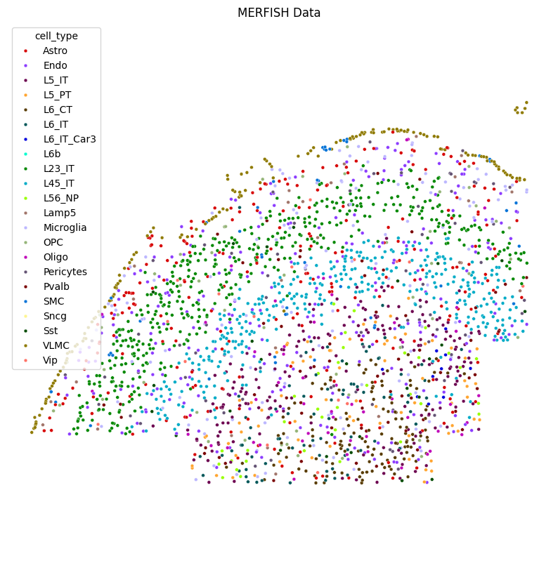
Plotting the Motor Cortex MERFISH
[9]:
plt.figure(figsize=(10,10))

sns.scatterplot(x = st_data.obsm['spatial'][st_data.obs['batch'] == 'mouse1_slice10'][:, 1],
                y = -st_data.obsm['spatial'][st_data.obs['batch'] == 'mouse1_slice10'][:, 0], legend = True,
                hue = st_data.obs['cell_type'][st_data.obs['batch'] == 'mouse1_slice10'],
                s = 12, palette = cell_type_palette)
plt.axis('equal')
plt.axis('off')
plt.title("MERFISH Data")
plt.show()
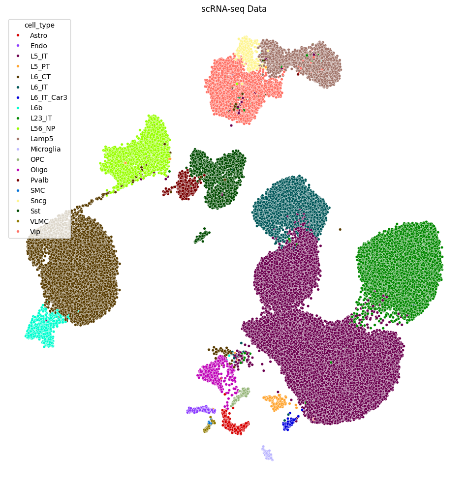
Plotting the Motor Cortex scRNAseq
[10]:
fit = umap.UMAP(
    n_neighbors = 100,
    min_dist = 0.8,
    n_components = 2,
)

sc_data.layers['log'] = np.log(sc_data.X + 1)
sc.pp.highly_variable_genes(sc_data, layer = 'log', n_top_genes = 2048)
sc_data.obsm['UMAP_exp'] = fit.fit_transform(np.log(sc_data[:, sc_data.var['highly_variable']].X + 1))
[11]:
fig = plt.figure(figsize = (10,10))
sns.scatterplot(x = sc_data.obsm['UMAP_exp'][:, 0], y = sc_data.obsm['UMAP_exp'][:, 1],  hue = sc_data.obs['cell_type'], s = 16,
                palette = cell_type_palette, legend = True)
plt.tight_layout()
plt.axis('off')
plt.title('scRNA-seq Data')
plt.show()
Running ENVI
We first define and ENVI model which computes the COVET matrices of the spatial data and intializes the CVAE:
[12]:
envi_model = scenvi.ENVI(spatial_data = st_data, sc_data = sc_data, covet_batch_size = 256)
Preparing gene sets for ENVI analysis...
Using pre-computed highly variable genes from single-cell data
Gene selection: 254 shared genes, 1832 unique to single-cell
Computing Niche Covariance Matrices
Using 64 pre-calculated highly variable genes for COVET
Calculating covariance matrices: 100%|██████████| 1081/1081 [00:04<00:00, 235.14it/s]
Computing matrix square roots: 100%|██████████| 1081/1081 [01:51<00:00,  9.72it/s]
Finished Initializing ENVI
Training ENVI and run auxiliary function
[13]:
envi_model.train()
envi_model.impute_genes()
envi_model.infer_niche_covet()
envi_model.infer_niche_celltype()
spatial: -6.316e-01 sc: -7.364e-01 cov: -5.564e-03 kl: 6.691e-01: 100%|██████████| 16000/16000 [02:37<00:00, 101.30it/s]
Computing latent representations
Encoding: 100%|██████████| 4322/4322 [01:33<00:00, 46.20it/s]
Encoding: 100%|██████████| 1113/1113 [00:23<00:00, 48.21it/s]
Imputing missing genes for spatial data
Decoding expression: 100%|██████████| 4322/4322 [01:32<00:00, 46.55it/s]
Infering niche COVET representation for single-cell data
Decoding covet: 100%|██████████| 1113/1113 [00:26<00:00, 41.61it/s]
Infering cell type niche composition for single cell data
Read ENVI predictions
[14]:
st_data.obsm['envi_latent'] = envi_model.spatial_data.obsm['envi_latent']
st_data.obsm['COVET'] = envi_model.spatial_data.obsm['COVET']
st_data.obsm['COVET_SQRT'] = envi_model.spatial_data.obsm['COVET_SQRT']
st_data.uns['COVET_genes'] =  envi_model.CovGenes
st_data.obsm['imputation'] = envi_model.spatial_data.obsm['imputation']
st_data.obsm['cell_type_niche'] = envi_model.spatial_data.obsm['cell_type_niche']

sc_data.obsm['envi_latent'] = envi_model.sc_data.obsm['envi_latent']
sc_data.obsm['COVET'] = envi_model.sc_data.obsm['COVET']
sc_data.obsm['COVET_SQRT'] = envi_model.sc_data.obsm['COVET_SQRT']
sc_data.obsm['cell_type_niche'] = envi_model.sc_data.obsm['cell_type_niche']
sc_data.uns['COVET_genes'] =  envi_model.CovGenes
Plot UMAPs of ENVI latent
Double Checking that cell types co-embed from the MERFISH and scRNA-seq datasets
[15]:
fit = umap.UMAP(
    n_neighbors = 100,
    min_dist = 0.3,
    n_components = 2,
)

latent_umap = fit.fit_transform(np.concatenate([st_data.obsm['envi_latent'], sc_data.obsm['envi_latent']], axis = 0))

st_data.obsm['latent_umap'] = latent_umap[:st_data.shape[0]]
sc_data.obsm['latent_umap'] = latent_umap[st_data.shape[0]:]
[16]:
lim_arr = np.concatenate([st_data.obsm['latent_umap'], sc_data.obsm['latent_umap']], axis = 0)


delta = 1
pre = 0.1
xmin = np.percentile(lim_arr[:, 0], pre) - delta
xmax = np.percentile(lim_arr[:, 0], 100 - pre) + delta
ymin = np.percentile(lim_arr[:, 1], pre) - delta
ymax = np.percentile(lim_arr[:, 1], 100 - pre) + delta
[17]:
fig = plt.figure(figsize = (13,5))
plt.subplot(121)
sns.scatterplot(x = sc_data.obsm['latent_umap'][:, 0],
                y = sc_data.obsm['latent_umap'][:, 1], hue = sc_data.obs['cell_type'], s = 8, palette = cell_type_palette,
                legend = False)
plt.title("scRNA-seq Latent")
plt.xlim([xmin, xmax])
plt.ylim([ymin, ymax])
plt.axis('off')

plt.subplot(122)
sns.scatterplot(x = st_data.obsm['latent_umap'][:, 0],
                y = st_data.obsm['latent_umap'][:, 1],  hue = st_data.obs['cell_type'], s = 8, palette = cell_type_palette, legend = True)


legend = plt.legend(title = 'Cell Type', prop={'size': 12}, fontsize = '12',  markerscale = 3, ncol = 2, bbox_to_anchor = (1, 1))#, loc = 'lower left')
plt.setp(legend.get_title(),fontsize='12')
plt.title("MERFISH Latent")
plt.axis('off')
plt.tight_layout()
plt.xlim([xmin, xmax])
plt.ylim([ymin, ymax])
plt.show()

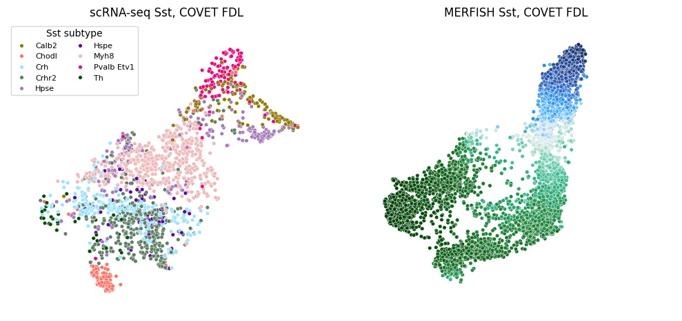
ENVI COVET analysis
Zooming on the Glutamatergic neuron, and using their COVET embedding for pseudo-depth prediction
[18]:
st_data_sst = st_data[st_data.obs['cell_type'] == 'Sst']
sc_data_sst = sc_data[sc_data.obs['cell_type'] == 'Sst']
[19]:
gran_sst_palette = {'Th': (0.0, 0.294118, 0.0, 1.0),
                    'Calb2': (0.560784, 0.478431, 0.0, 1.0),
                    'Chodl': (1.0, 0.447059, 0.4, 1.0),
                    'Myh8': (0.933333, 0.72549, 0.72549, 1.0),
                    'Crhr2': (0.368627, 0.494118, 0.4, 1.0),
                    'Hpse': (0.65098, 0.482353, 0.72549, 1.0),
                    'Hspe': (0.352941, 0.0, 0.643137, 1.0),
                    'Crh': (0.607843, 0.894118, 1.0, 1.0),
                    'Pvalb Etv1': (0.92549, 0.0, 0.466667, 1.0)}
Calculating FDL and DC on COVET
Note that we are running FDL on COVET_SQRT, this is because the distance between COVET matrices is the L2 between their SQRT. We can simply run FDL (or DC, UMAP, PhenoGraph, etc.) on the COVET_SQRT to analyize COVET niche representation!
[20]:
import scipy.sparse
[21]:
def flatten(x):
    return(x.reshape([x.shape[0], -1]))

def run_diffusion_maps(data_df, n_components=10, knn=30, alpha=0):
    """Run Diffusion maps using the adaptive anisotropic kernel
    :param data_df: PCA projections of the data or adjacency matrix
    :param n_components: Number of diffusion components
    :param knn: Number of nearest neighbors for graph construction
    :param alpha: Normalization parameter for the diffusion operator
    :return: Diffusion components, corresponding eigen values and the diffusion operator
    """

    # Determine the kernel
    N = data_df.shape[0]

    if(type(data_df).__module__ == np.__name__):
        data_df = pd.DataFrame(data_df)

    if not scipy.sparse.issparse(data_df):
        print("Determing nearest neighbor graph...")
        temp = sc.AnnData(data_df.values)
        sc.pp.neighbors(temp, n_pcs=0, n_neighbors=knn)
        kNN = temp.obsp['distances']

        # Adaptive k
        adaptive_k = int(np.floor(knn / 3))
        adaptive_std = np.zeros(N)

        for i in np.arange(len(adaptive_std)):
            adaptive_std[i] = np.sort(kNN.data[kNN.indptr[i] : kNN.indptr[i + 1]])[
                adaptive_k - 1
            ]

        # Kernel
        x, y, dists = scipy.sparse.find(kNN)

        # X, y specific stds
        dists = dists / adaptive_std[x]
        W = scipy.sparse.csr_matrix((np.exp(-dists), (x, y)), shape=[N, N])

        # Diffusion components
        kernel = W + W.T
    else:
        kernel = data_df

    # Markov
    D = np.ravel(kernel.sum(axis=1))

    if alpha > 0:
        # L_alpha
        D[D != 0] = D[D != 0] ** (-alpha)
        mat = scipy.sparse.csr_matrix((D, (range(N), range(N))), shape=[N, N])
        kernel = mat.dot(kernel).dot(mat)
        D = np.ravel(kernel.sum(axis=1))

    D[D != 0] = 1 / D[D != 0]
    T = scipy.sparse.csr_matrix((D, (range(N), range(N))), shape=[N, N]).dot(kernel)
    # Eigen value dcomposition
    D, V = scipy.sparse.linalg.eigs(T, n_components, tol=1e-4, maxiter=1000)
    D = np.real(D)
    V = np.real(V)
    inds = np.argsort(D)[::-1]
    D = D[inds]
    V = V[:, inds]

    # Normalize
    for i in range(V.shape[1]):
        V[:, i] = V[:, i] / np.linalg.norm(V[:, i])

    return V[:, 1:]
[22]:
fit = umap.UMAP(
    n_neighbors = 30,
    min_dist = 0.1,
    n_components = 2,
)

UMAP_COVET = fit.fit_transform(np.concatenate([flatten(st_data_sst.obsm['COVET_SQRT']),
                                               flatten(sc_data_sst.obsm['COVET_SQRT'])], axis = 0))

st_data_sst.obsm['UMAP_COVET'] = UMAP_COVET[:st_data_sst.shape[0]]
sc_data_sst.obsm['UMAP_COVET'] = UMAP_COVET[st_data_sst.shape[0]:]
[23]:
DC_COVET = run_diffusion_maps(np.concatenate([flatten(st_data_sst.obsm['COVET_SQRT']),
                                              flatten(sc_data_sst.obsm['COVET_SQRT'])], axis = 0))

st_data_sst.obsm['DC_COVET'] = DC_COVET[:st_data_sst.shape[0]]
sc_data_sst.obsm['DC_COVET'] = DC_COVET[st_data_sst.shape[0]:]
Determing nearest neighbor graph...
Reverse DC if needed
DC direction is arbitrary; so flip DC direction if it’s backwards
Should go from blue (shallow) to green (deep)
[ ]:
st_data_sst.obsm['DC_COVET'] = -DC_COVET[:st_data_sst.shape[0]]
sc_data_sst.obsm['DC_COVET'] = -DC_COVET[st_data_sst.shape[0]:]
Plot DC and Depth
[24]:
lim_arr = np.concatenate([st_data_sst.obsm['UMAP_COVET'], sc_data_sst.obsm['UMAP_COVET']], axis = 0)


delta = 1
pre = 0.01
xmin = np.percentile(lim_arr[:, 0], pre) - delta
xmax = np.percentile(lim_arr[:, 0], 100 - pre) + delta
ymin = np.percentile(lim_arr[:, 1], pre) - delta
ymax = np.percentile(lim_arr[:, 1], 100 - pre) + delta
[25]:
plt.figure(figsize=(10,5))

plt.subplot(121)
sns.scatterplot(x = sc_data_sst.obsm['UMAP_COVET'][:, 0],
                y = sc_data_sst.obsm['UMAP_COVET'][:, 1],
                hue = sc_data_sst.obs['cluster_label'], s = 16,  palette= gran_sst_palette, legend = True)
plt.tight_layout()
plt.xlim([xmin, xmax])
plt.ylim([ymin, ymax])
plt.title('scRNA-seq Sst, COVET FDL')
legend = plt.legend(title = 'Sst subtype', prop={'size': 8}, fontsize = '8',  markerscale = 1, ncol = 2)
plt.axis('off')

plt.subplot(122)
ax = sns.scatterplot(x = st_data_sst.obsm['UMAP_COVET'][:, 0],
                y = st_data_sst.obsm['UMAP_COVET'][:, 1],
                c = st_data_sst.obsm['DC_COVET'][:,0], s = 16,  cmap= 'cet_CET_D13', legend = False)
plt.tight_layout()
plt.xlim([xmin, xmax])
plt.ylim([ymin, ymax])
plt.axis('off')
plt.title('MERFISH Sst, COVET FDL')
plt.show()
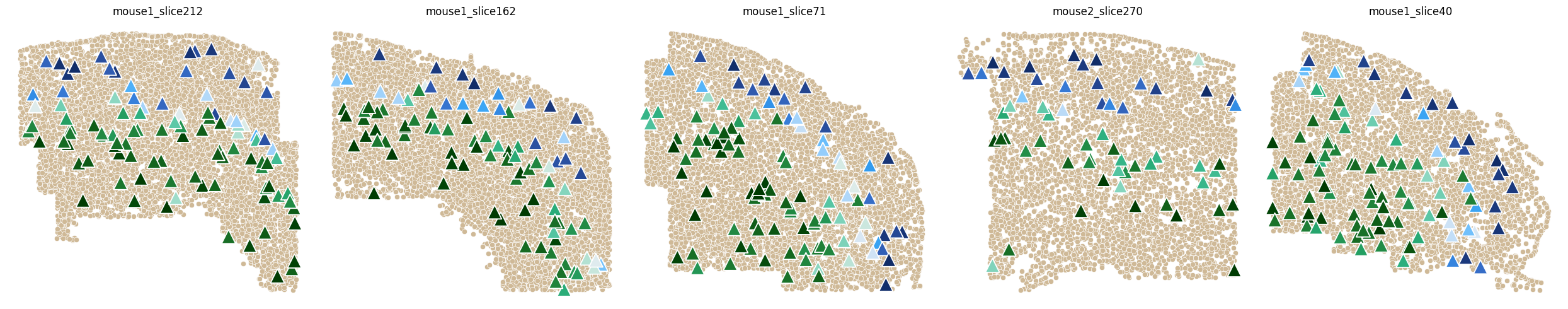
[26]:
fig = plt.figure(figsize=(25,5))

for ind, batch in enumerate(['mouse1_slice212', 'mouse1_slice162', 'mouse1_slice71', 'mouse2_slice270', 'mouse1_slice40']):
    st_dataBatch = st_data[st_data.obs['batch'] == batch]
    st_dataPlotBatch = st_data_sst[st_data_sst.obs['batch'] == batch]

    plt.subplot(1,5, 1+ ind)
    sns.scatterplot(x = st_dataBatch.obsm['spatial'][:, 0], y = st_dataBatch.obsm['spatial'][:, 1],  color = (207/255,185/255,151/255, 1))
    sns.scatterplot(x = st_dataPlotBatch.obsm['spatial'][:, 0], y = st_dataPlotBatch.obsm['spatial'][:, 1], marker = '^',
                        c = st_dataPlotBatch.obsm['DC_COVET'][:, 0], s = 256,  cmap= 'cet_CET_D13', legend = False)
    plt.title(batch)
    plt.axis('off')
    plt.tight_layout()

plt.show()
Subtype Depth
Box plot of cortical depth for each cell in every subtype
[27]:
depth_df = pd.DataFrame()
depth_df['Subtype'] = sc_data_sst.obs['cluster_label']
depth_df['Depth'] = -sc_data_sst.obsm['DC_COVET'][:,0]
[28]:
subtype_depth_order = depth_df.groupby(['Subtype']).mean().sort_values(by = 'Depth', ascending=False).index
[29]:
plt.figure(figsize=(12,5))
sns.set(font_scale=1.7)
sns.set_style("whitegrid")
sns.boxenplot(depth_df, x = 'Subtype', y = 'Depth',# bw = 1, width = 0.9,
          order = subtype_depth_order,
          palette = gran_sst_palette)
plt.tight_layout()
plt.show()

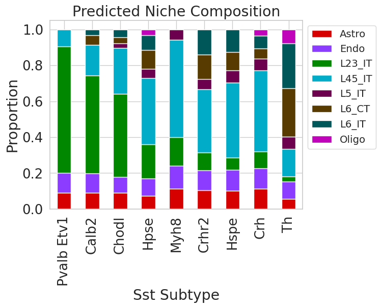
Niche Cell Type Composition
ENVI uses COVET to predict the niche cell type abundence for each scRNA-seq cell. For each Sst subtype, we will compute the canonical niche composition:
[30]:
subtype_canonical = pd.DataFrame([sc_data_sst[sc_data_sst.obs['cluster_label']==subtype].obsm['cell_type_niche'].mean(axis = 0) for subtype in subtype_depth_order],
                                     index = subtype_depth_order, columns = sc_data.obsm['cell_type_niche'].columns)
[31]:
subtype_canonical[subtype_canonical<0.2] = 0
subtype_canonical.drop(labels=subtype_canonical.columns[(subtype_canonical == 0).all()], axis=1, inplace=True)
subtype_canonical = subtype_canonical.div(subtype_canonical.sum(axis=1), axis=0)
Plot as Stacked Bar Plots
[32]:
subtype_canonical.plot(kind = 'bar', stacked = 'True',
                       color = {col:cell_type_palette[col] for col in subtype_canonical.columns})
plt.legend(bbox_to_anchor = (1,1), ncols = 1, fontsize = 'x-small')
plt.title("Predicted Niche Composition")
plt.ylabel("Proportion")
plt.xlabel("Sst Subtype")
plt.show()
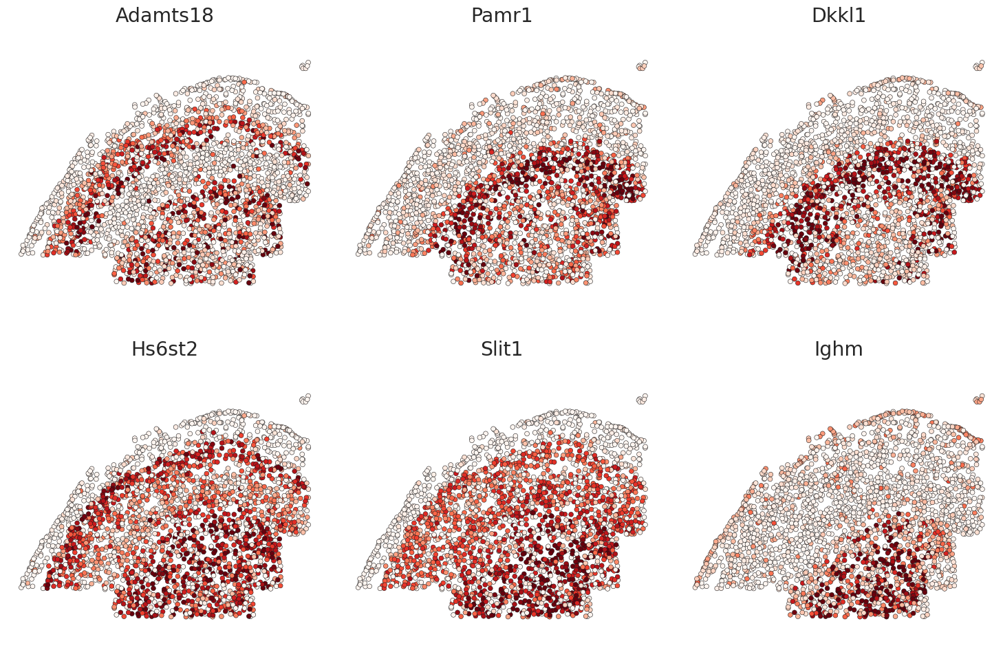
ENVI imputation on Spatial Data
[33]:
tick_genes = np.asarray(['Adamts18','Pamr1', 'Dkkl1', 'Hs6st2', 'Slit1', 'Ighm'])
[34]:
plt.figure(figsize=(15,10))

for ind, gene in enumerate(tick_genes):
    plt.subplot(2,3,1+ind)

    cvec = np.log(st_data[st_data.obs['batch'] == 'mouse1_slice10'].obsm['imputation'][gene] + 0.1)
    sns.scatterplot(x = st_data.obsm['spatial'][st_data.obs['batch'] == 'mouse1_slice10'][:, 1],
                    y = -st_data.obsm['spatial'][st_data.obs['batch'] == 'mouse1_slice10'][:, 0], legend = False,
                    c = cvec, cmap = 'Reds',
                    vmax = np.percentile(cvec, 95), vmin = np.percentile(cvec, 30),
                    s = 24, edgecolor = 'k')#, palette = cell_type_palette)
    plt.title(gene)
    plt.axis('equal')
    plt.axis('off')
    plt.tight_layout()
plt.show()